Case 1: Search Autocompletion
1. Business Problem Statement
Building a fast, scalable autocomplete system that predicts and suggests relevant queries instantly as users type, handling billions of searches globally with high accuracy.
Domain: Search Engines, Information Retrieval, User Experience
2. Challenges
- Handling billions of daily searches at a global scale.
- Delivering suggestions within milliseconds for seamless experience.
- Incorporating trending and fresh queries quickly.
- Supporting typos, slang, and multilingual inputs.
3. Algorithms involved
- Weighted Finite State Transducers (WFST)-- Compact, efficient representation of query dictionaries for prefix matching.
- Trie (Prefix Tree) -- Fast prefix lookups for query suggestions.
- Ternary Search Tree -- Space-optimized string storage and retrieval.
- Frequency Counting / Heuristics -- Popularity, recency, and user behavior-based scoring.
- Fuzzy Matching Algorithms (e.g., Levenshtein distance) -- Handle typos and spelling variations.
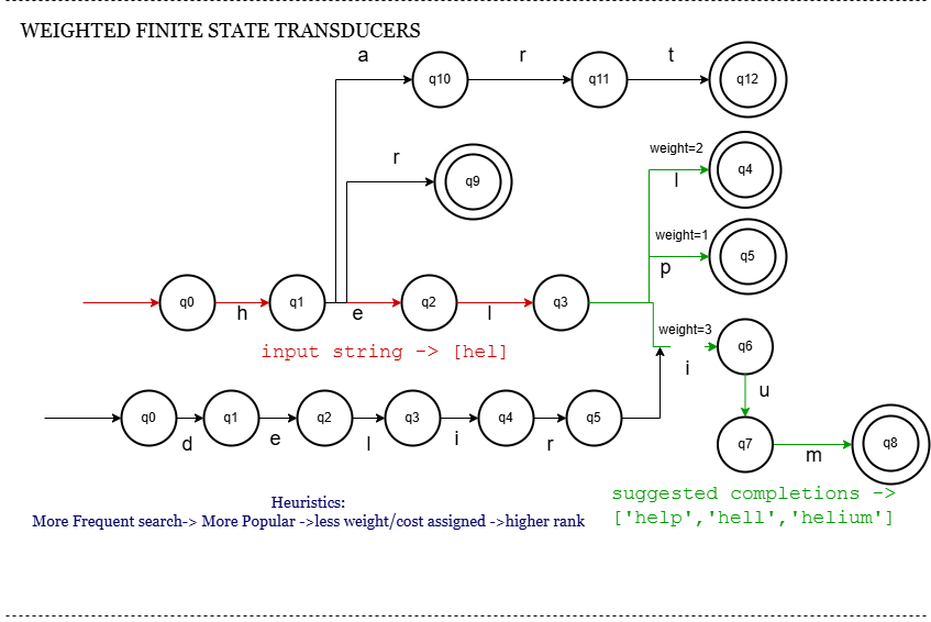
1] Weighted Finite State Transducer (Weighted FST)
What it is?
A Weighted FST is a deterministic finite automaton extended with weights on transitions or states, mapping input strings (query prefixes) to outputs (full queries or scores), commonly used in large-scale autocomplete.
How does it work?
- Input string is processed state by state.
- Transitions labeled with input characters guide traversal.
- Weights encode frequency/popularity, enabling ranking.
- Minimization merges equivalent states, compressing data.
- Outputs top suggestions with associated weights quickly.
Workflow
5. Code Snippet
class WFSTNode:
    def __init__(self):
        self.transitions = {}  # char -> (node, weight)
        self.is_final = False
        self.output = None

class WeightedFST:
    def __init__(self):
        self.root = WFSTNode()

    def insert(self, word, weight):
        node = self.root
        for char in word:
            if char not in node.transitions:
                node.transitions[char] = (WFSTNode(), 0)
            next_node, _ = node.transitions[char]
            node.transitions[char] = (next_node, weight)
            node = next_node
        node.is_final = True
        node.output = word

    def autocomplete(self, prefix):
        node = self.root
        for char in prefix:
            if char not in node.transitions:
                return []
            node, _ = node.transitions[char]
        return self._collect(node, prefix)

    def _collect(self, node, prefix):
        results = []
        stack = [(node, prefix)]
        while stack:
            cur, pre = stack.pop()
            if cur.is_final:
                results.append(pre)
            for c, (nxt, w) in cur.transitions.items():
                stack.append((nxt, pre + c))
        # Normally sort by weights, simplified here
        return results

# Example usage
wfst = WeightedFST()
wfst.insert("hello", weight=1)    # Most popular
wfst.insert("help", weight=2)
wfst.insert("helium", weight=3)
wfst.insert("hero", weight=4)
wfst.insert("man", weight=10)
wfst.insert("genre", weight=8)
wfst.insert("gentle", weight=6)
wfst.insert("gem", weight=5)

print(wfst.autocomplete("ge"))
print(wfst.autocomplete("he"))
print(wfst.autocomplete("hel"))

OUTPUT:
    ['gem', 'gentle', 'genre']
    ['hello', 'help', 'helium', 'hero']
    ['hello', 'help', 'helium']
Efficiency Analysis
- Time: O(m) for prefix traversal (m = prefix length)
- Space:Highly compact due to minimization
- Ranking:Built-in weights enable fast top suggestions
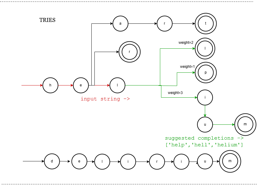
2] Trie
What it is?
A Trie is a tree-like data structure where each edge corresponds to a character; nodes represent prefixes. Commonly used for exact prefix matching.
How does it work?
- Insert words character-by-character along tree edges.
- Each node represents a prefix.
- Search traverses nodes following input characters.
- Suggestions are collected from subtree nodes.
Workflow
5. Code Snippet
class TrieNode:
    def __init__(self):
        self.children = {}
        self.is_end = False

class Trie:
    def __init__(self):
        self.root = TrieNode()

    def insert(self, word):
        node = self.root
        for char in word:
            node = node.children.setdefault(char, TrieNode())
        node.is_end = True

    def autocomplete(self, prefix):
        node = self.root
        for char in prefix:
            if char not in node.children:
                return []
            node = node.children[char]
        return self._collect(node, prefix)

    def _collect(self, node, prefix):
        results = []
        if node.is_end:
            results.append(prefix)
        for c, nxt in node.children.items():
            results.extend(self._collect(nxt, prefix + c))
        return results


# Example usage
trie = Trie()
trie.insert("hello", {"definition": "a greeting"})
trie.insert("help", {"definition": "to assist"})
trie.insert("helium", {"definition": "an element"})
trie.insert("hear", {"definition": "to listen"})
print(trie.findWordsWithPrefix("hel"))

OUTPUT:
    [('hello', {'definition': 'a greeting'}),
     ('help', {'definition': 'to assist'}),
     ('helium', {'definition': 'an element'})]
Efficiency Analysis
- Time: O(m + k) for prefix + collecting k suggestions
- Space:Larger than FST (stores all nodes explicitly)
- Ranking:No built-in ranking, requires extra data structures
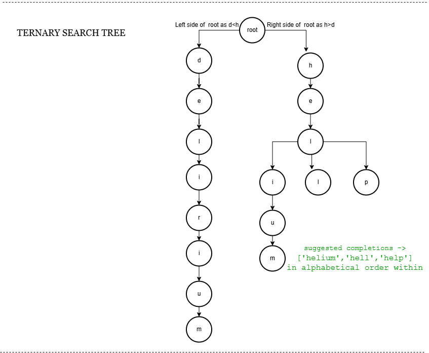
3] Ternary Search Tree (TST)
What it is?
A TST is a hybrid between binary search trees and tries: each node stores a character and has three children (left, middle, right) for lex order navigation and sequence continuation.
How does it work?
- Each node compares character:
- Left: characters less than current
- Middle: next char in word if equal
- Right: characters greater than current
- Insert and search use these comparisons.
- Autocomplete collects words below prefix node.
Workflow
5. Code Snippet
class TSTNode:
    def __init__(self, char):
        self.char = char
        self.left = self.mid = self.right = None
        self.is_end = False

class TST:
    def __init__(self):
        self.root = None

    def insert(self, word):
        def _insert(node, word, i):
            c = word[i]
            if not node:
                node = TSTNode(c)
            if c < node.char:
                node.left = _insert(node.left, word, i)
            elif c > node.char:
                node.right = _insert(node.right, word, i)
            else:
                if i + 1 == len(word):
                    node.is_end = True
                else:
                    node.mid = _insert(node.mid, word, i+1)
            return node
        self.root = _insert(self.root, word, 0)

    def autocomplete(self, prefix):
        def _search(node, word, i):
            if not node:
                return None
            c = word[i]
            if c < node.char:
                return _search(node.left, word, i)
            elif c > node.char:
                return _search(node.right, word, i)
            else:
                if i + 1 == len(word):
                    return node
                return _search(node.mid, word, i+1)

        def _collect(node, pre, results):
            if not node:
                return
            _collect(node.left, pre, results)
            if node.is_end:
                results.append(pre + node.char)
            _collect(node.mid, pre + node.char, results)
            _collect(node.right, pre, results)

        results = []
        node = _search(self.root, prefix, 0)
        if not node:
            return results
        if node.is_end:
            results.append(prefix)
        _collect(node.mid, prefix, results)
        return results


# Example usage
tst = TST()
words = ["hello", "help", "helium", "hero", "her", "heat", "delirium"]
for word in words:
    tst.insert(word)

print(tst.autocomplete("her"))
print(tst.autocomplete("hel"))
print(tst.autocomplete("h"))

OUTPUT:
    ['her', 'hero']
    ['helium', 'hello', 'help']
    ['heat', 'helium', 'hello', 'help', 'her', 'hero']
Efficiency Analysis
- Time: O(m + k) with balanced character comparisons
- Space:More compact than Trie, less than FST
- Ranking:No built-in weights, extra storage needed
Case study Summary
| Sl.no. | Algorithm | Time Complexity (Prefix Query) | Space Efficiency | Ranking Support | Notable difference | Suitability for Google Search Autocomplete |
|---|---|---|---|---|---|---|
| 1 | Weighted FST | O(m) | Very high (compressed) | Built-in weights | Saves memory and transition steps by minimizing processing of duplicate suffixes. | Best: Scales to billions of queries efficiently |
| 2 | Trie | O(m + k) | High (large memory) | No native weights | Looks like a tree of prefixes with no alphavetical ordering. | Simple but memory-heavy for huge data |
| 3 | Ternary Search Tree | O(m + k) | Moderate | No native weights | Looks like a binary search tree for characters, but also stores sequences like a trie. | Balanced but less optimal for Google's scale as it's less compact and slower |
Case 2: Route Assessment
1. Business Problem Statement
Build a scalable system to assess and recommend optimal real-time travel routes across various transport modes.
Domain: Navigation Systems, Traffic Optimization, Real-Time Systems
2. Challenges
- Collecting accurate real-time traffic data from billions of users.
- Dynamically updating routes during live traffic changes.
- Scaling to handle billions of global route requests.
- Adapting routes to regional traffic rules and landmarks.
- Personalizing routes based on user preferences.
- Predicting accurate ETAs using real-time + historical data.
- Ensuring low-latency route computation globally.
3. Algorithms Involved
- Dijkstra’s Algorithm – Solves shortest path efficiently in static road networks.
- A* Algorithm – Enhances Dijkstra’s with heuristics for faster pathfinding.
- Contraction Hierarchies – Preprocesses road networks to enable faster route queries using shortcuts.
- R-Tree / Quad Tree – Used for efficient spatial indexing of nearby roads, landmarks, and intersections.
- Ford-Fulkerson / Max Flow – Models and analyzes traffic capacity and congestion zones.
- Bayesian Networks / Time-Series Analysis – Predicts future traffic patterns using historical and real-time data.
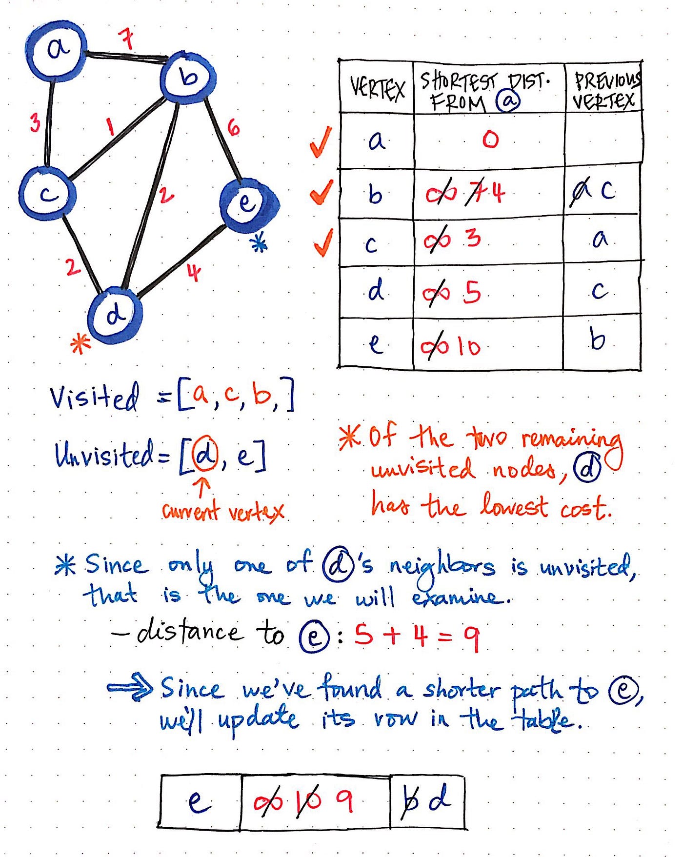
1] Dijkstra’s Algorithm
What it is?
An algorithm for finding the shortest path from a source node to all other nodes in a weighted graph with non-negative weights.
How does it work?
- Start from a source node.
- Initialize distances to all nodes as infinity except the source (0).
- Use a min-heap (priority queue) for efficient retrieval of the next closest node.
- Relax edges: update neighbor distances if a shorter path is found.
- Mark nodes as visited to avoid reprocessing.
- Repeat until all nodes are visited.
Workflow
5. Code Snippet
class Graph():

    def __init__(self, vertices):
        self.V = vertices
        self.graph = [[0 for column in range(vertices)]
                      for row in range(vertices)]

    def printSolution(self, dist):
        print("Vertex \t Distance from Source")
        for node in range(self.V):
            print(node, "\t\t", dist[node])

    # A utility function to find the vertex with
    # minimum distance value, from the set of vertices
    # not yet included in shortest path tree
    def minDistance(self, dist, sptSet):

        # Initialize minimum distance for next node
        min = 1e7

        # Search not nearest vertex not in the
        # shortest path tree
        for v in range(self.V):
            if dist[v] < min and sptSet[v] == False:
                min = dist[v]
                min_index = v

        return min_index

    # Function that implements Dijkstra's single source
    # shortest path algorithm for a graph represented
    # using adjacency matrix representation
    def dijkstra(self, src):

        dist = [1e7] * self.V
        dist[src] = 0
        sptSet = [False] * self.V

        for cout in range(self.V):

            # Pick the minimum distance vertex from
            # the set of vertices not yet processed.
            # u is always equal to src in first iteration
            u = self.minDistance(dist, sptSet)

            # Put the minimum distance vertex in the
            # shortest path tree
            sptSet[u] = True

            # Update dist value of the adjacent vertices
            # of the picked vertex only if the current
            # distance is greater than new distance and
            # the vertex in not in the shortest path tree
            for v in range(self.V):
                if (self.graph[u][v] > 0 and
                   sptSet[v] == False and
                   dist[v] > dist[u] + self.graph[u][v]):
                    dist[v] = dist[u] + self.graph[u][v]

        self.printSolution(dist)

# Driver program
g = Graph(9)
g.graph = [[0, 4, 0, 0, 0, 0, 0, 8, 0],
           [4, 0, 8, 0, 0, 0, 0, 11, 0],
           [0, 8, 0, 7, 0, 4, 0, 0, 2],
           [0, 0, 7, 0, 9, 14, 0, 0, 0],
           [0, 0, 0, 9, 0, 10, 0, 0, 0],
           [0, 0, 4, 14, 10, 0, 2, 0, 0],
           [0, 0, 0, 0, 0, 2, 0, 1, 6],
           [8, 11, 0, 0, 0, 0, 1, 0, 7],
           [0, 0, 2, 0, 0, 0, 6, 7, 0]
           ]

g.dijkstra(0)

OUTPUT:
Vertex 	 Distance from Source
0 		 0
1 		 4
2 		 12
3 		 19
4 		 21
5 		 11
6 		 9
7 		 8
8 		 14
Efficiency Analysis
- Time: O((V + E) log V)
- Space:O(V)
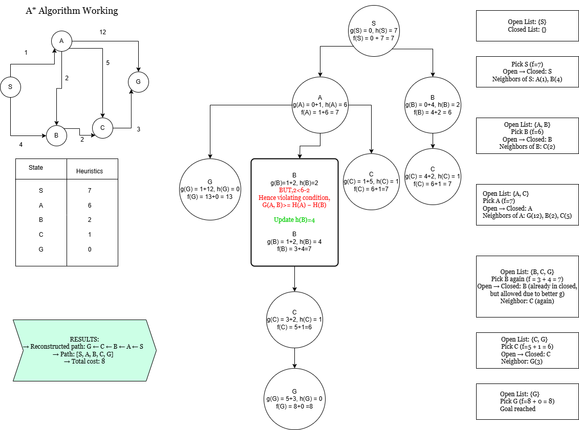
2] A* Algorithm
What it is?
An informed search algorithm that finds the shortest path using heuristics.
How does it work?
- Initializes open and closed sets.
- Pick node with lowest f(n).
- Relax neighbours using a cost function: f(n) = g(n) + h(n):
- g(n): actual distance
- h(n): heuristic estimate
- Repeat until goal is reached.
Workflow
5. Code Snippet
class Graph:
    def __init__(self, adjacency_list):
        self.adjacency_list = adjacency_list

    def get_neighbors(self, v):
        return self.adjacency_list.get(v, [])

    def h(self, n):
        H = {
            'S': 7,
            'A': 6,
            'B': 2,
            'C': 1,
            'G': 0
        }
        return H[n]

    def a_star_algorithm(self, start_node, stop_node):
        open_list = set([start_node])
        closed_list = set([])

        g = {start_node: 0}
        parents = {start_node: start_node}

        while open_list:
            n = None
            for v in open_list:
                if n is None or g[v] + self.h(v) < g[n] + self.h(n):
                    n = v

            if n is None:
                print('Path does not exist!')
                return None

            if n == stop_node:
                reconst_path = []
                while parents[n] != n:
                    reconst_path.append(n)
                    n = parents[n]
                reconst_path.append(start_node)
                reconst_path.reverse()
                print('Path found: {}'.format(reconst_path))
                print('Total cost: {}'.format(g[stop_node]))
                return reconst_path

            for (m, weight) in self.get_neighbors(n):
                if m not in open_list and m not in closed_list:
                    open_list.add(m)
                    parents[m] = n
                    g[m] = g[n] + weight
                else:
                    if g[m] > g[n] + weight:
                        g[m] = g[n] + weight
                        parents[m] = n
                        if m in closed_list:
                            closed_list.remove(m)
                            open_list.add(m)

            open_list.remove(n)
            closed_list.add(n)

        print('Path does not exist!')
        return None


# Custom graph from your input
adjacency_list = {
    'S': [('A', 1), ('B', 4)],
    'A': [('G', 12), ('B', 2), ('C', 5)],
    'B': [('C', 2)],
    'C': [('G', 3)]
}

graph1 = Graph(adjacency_list)
graph1.a_star_algorithm('S', 'G')

OUTPUT:
Path found: ['S', 'A', 'B', 'C', 'G']
Total cost: 8
['S', 'A', 'B', 'C', 'G']
Efficiency Analysis
- Time: O(V^2) [O((V+E)log V) if min-heap (priority queue used)
- Space:O(V)
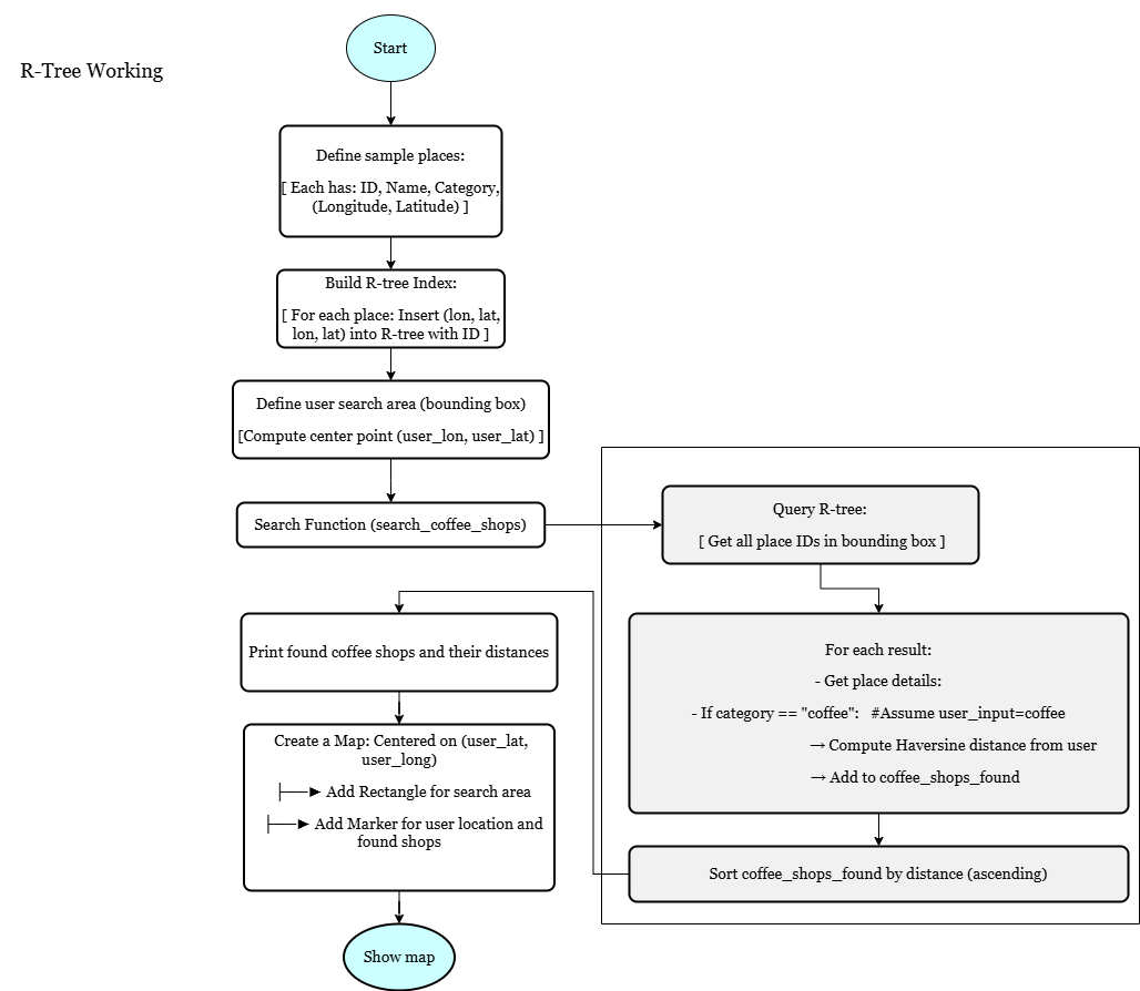
3] R-Tree
What it is?
Spatial data structure used for efficiently indexing multi-dimensional information like maps.
How does it work?
- R-Tree: groups nearby objects using bounding rectangles.
- Insert: add object by checking overlapping regions.
- Query: search through relevant nodes only.
Workflow
5. Code Snippet
from rtree import index
from math import radians, cos, sin, asin, sqrt
import folium

# Haversine distance function (km)
def haversine(lon1, lat1, lon2, lat2):
    lon1, lat1, lon2, lat2 = map(radians, [lon1, lat1, lon2, lat2])
    dlon = lon2 - lon1
    dlat = lat2 - lat1
    a = sin(dlat/2)**2 + cos(lat1) * cos(lat2) * sin(dlon/2)**2
    c = 2 * asin(sqrt(a))
    r = 6371
    return c * r

# Sample places: id -> (name, category, (lon, lat))
places = {
    1: ("Coffee Shop A", "coffee", (77.59, 12.97)),
    2: ("Bookstore", "bookstore", (77.58, 12.95)),
    3: ("Coffee Shop B", "coffee", (77.60, 12.96)),
    4: ("Museum", "museum", (77.55, 12.92)),
    5: ("Coffee Shop C", "coffee", (77.62, 12.99)),  # Outside search area
    6: ("Gym", "gym", (77.61, 12.94)),
    7: ("Coffee Shop D", "coffee", (77.56, 12.93)),  # Outside search area
}

# Build R-tree index
idx = index.Index()
for place_id, (name, category, (x, y)) in places.items():
    idx.insert(place_id, (x, y, x, y))

# User inputs search bounding box: (min_lon, min_lat, max_lon, max_lat)
user_search_area = (77.57, 12.94, 77.61, 12.98)
user_lon = (user_search_area[0] + user_search_area[2]) / 2
user_lat = (user_search_area[1] + user_search_area[3]) / 2

# Search coffee shops inside area and calculate distances
def search_coffee_shops(index_obj, search_area, user_lon, user_lat):
    print(f"Searching coffee shops inside area: {search_area}")
    results = list(index_obj.intersection(search_area))

    coffee_shops_found = []
    for place_id in results:
        name, category, (lon, lat) = places[place_id]
        if category == "coffee":
            dist = haversine(user_lon, user_lat, lon, lat)
            coffee_shops_found.append((name, (lon, lat), dist))

    coffee_shops_found.sort(key=lambda x: x[2])

    if not coffee_shops_found:
        print("No coffee shops found in the search area.")
    else:
        print(f"Found {len(coffee_shops_found)} coffee shop(s):")
        for name, coord, dist in coffee_shops_found:
            print(f"- {name} at {coord}, Distance: {dist:.2f} km")
    return coffee_shops_found

coffee_shops = search_coffee_shops(idx, user_search_area, user_lon, user_lat)

# Create interactive map
m = folium.Map(location=[user_lat, user_lon], zoom_start=14)

# Draw search area rectangle
bounds = [(user_search_area[1], user_search_area[0]), (user_search_area[3], user_search_area[2])]
folium.Rectangle(bounds=bounds, color="blue", fill=True, fill_opacity=0.1, tooltip="Search Area").add_to(m)

# Mark user location
folium.Marker(
    location=[user_lat, user_lon],
    popup="User Search Center",
    icon=folium.Icon(color='green', icon='user')
).add_to(m)

# Mark coffee shops on map
for name, (lon, lat), dist in coffee_shops:
    folium.Marker(
        location=[lat, lon],
        popup=f"{name}
Distance: {dist:.2f} km",
        icon=folium.Icon(color='red', icon='coffee', prefix='fa')
    ).add_to(m)

# Show the map
m

OUTPUT:
Searching coffee shops inside area: (77.57, 12.94, 77.61, 12.98)
Found 2 coffee shop(s):
- Coffee Shop B at (77.6, 12.96), Distance: 1.08 km
- Coffee Shop A at (77.59, 12.97), Distance: 1.11 km
Efficiency Analysis
- Time: O(log n) insert/search
- Space:O(n)
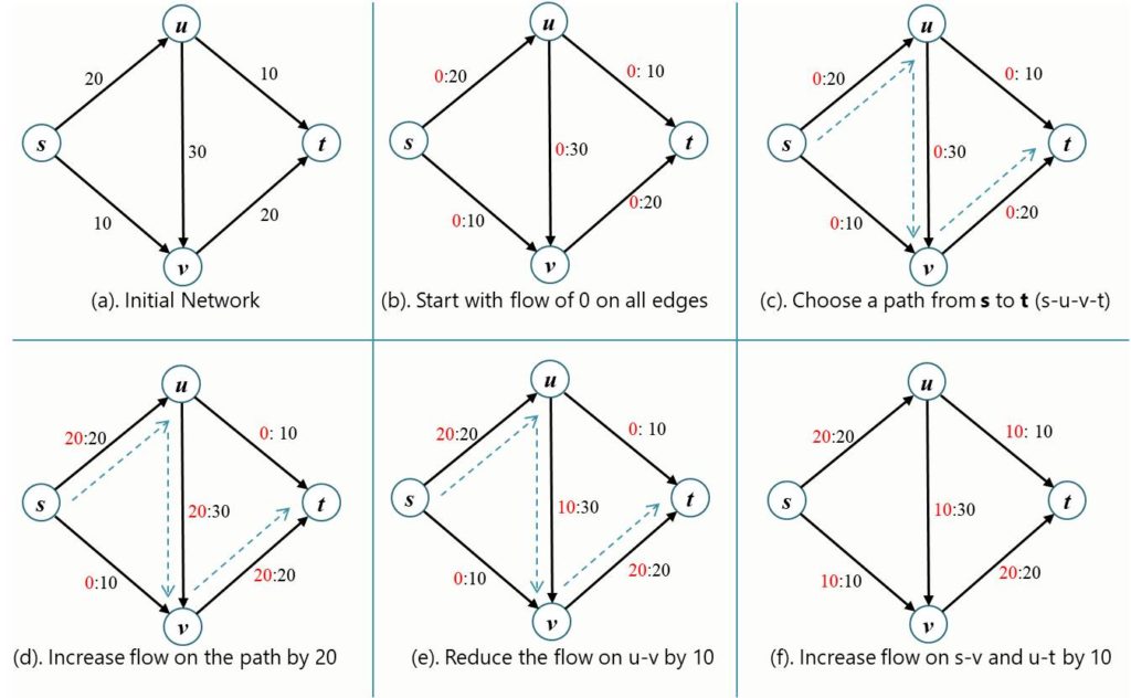
4] Ford-Fulkerson / Max Flow
What it is?
Finds the maximum flow from source to sink in a flow network.
How does it work?
- Augment flow along a path until no more augmenting paths are found.
- Initialize flow to 0.
- While there’s an augmenting path:
- Find min capacity on path
- Update residual graph
Workflow
5. Code Snippet
from collections import defaultdict

class Graph:
    def __init__(self, vertices):
        self.graph = defaultdict(dict)
        self.V = vertices

    def add_edge(self, u, v, capacity):
        self.graph[u][v] = capacity
        if u not in self.graph[v]:
            self.graph[v][u] = 0

    def _dfs(self, s, t, visited, path):
        visited.add(s)
        if s == t:
            return path
        for neighbor in self.graph[s]:
            if neighbor not in visited and self.graph[s][neighbor] > 0:
                result = self._dfs(neighbor, t, visited, path + [(s, neighbor)])
                if result:
                    return result
        return None

    def ford_fulkerson(self, source, sink):
        max_flow = 0
        while True:
            visited = set()
            path = self._dfs(source, sink, visited, [])
            if not path:
                break

            flow = min(self.graph[u][v] for u, v in path)

            for u, v in path:
                self.graph[u][v] -= flow
                self.graph[v][u] += flow

            max_flow += flow
            print(f"Augmenting path: {path}, flow: {flow}")
        return max_flow

g=Graph(4)
g.add_edge('s','u',20)
g.add_edge('s','v',10)
g.add_edge('u','v',30)
g.add_edge('u','t',10)
g.add_edge('v','t',20)

max_flow = g.ford_fulkerson('s', 't')
print(f"Max Flow: {max_flow}")

OUTPUT:
Augmenting path: [('s', 'u'), ('u', 'v'), ('v', 't')], flow: 20
Augmenting path: [('s', 'v'), ('v', 'u'), ('u', 't')], flow: 10
Max Flow: 30
Efficiency Analysis
- Time: O(E * max flow)
- Space: O(V^2)
Case Study Summary
| Sl.no. | Algorithm | Time Complexity (Prefix Query) | Space Efficiency | Notable Difference | Suitability for Use Case |
|---|---|---|---|---|---|
| 1 | Dijkstra | O((V + E) log V) | Moderate | Finds shortest paths using greedy strategy and priority queues. | Ideal for maps and route optimization. |
| 2 | A* Search | O((V + E) log V) | Moderate | Enhances Dijkstra by using heuristics to guide search toward goal faster. | Best for pathfinding with target-aware optimization (e.g., GPS). |
| 3 | R-tree | O(log n) | High (compact for spatial data) | Index structure for spatial data using bounding rectangles. | Excellent for geo-search like "coffee near me". |
| 4 | Ford-Fulkerson | O(max_flow × E) | Low to Moderate | Uses DFS/BFS to find augmenting paths in residual graph for max flow. | Best for flow problems (networks, logistics). |
Case 3: Data Storage and Indexing
1. Business Problem Statement
To efficiently store and index billions of web pages to support fast, relevant, and scalable search queries across the globe
Domain: Search Engines, Big Data, Distributed Systems, Information Retrieval
2. Challenges
- Storing and managing billions of web pages efficiently at scale.
- Building and updating inverted indexes quickly over distributed data.
- Delivering low-latency search results within milliseconds.
- Reducing storage needs through compression and deduplication.
3. Algorithms Involved
- B-trees – optimize disk-based storage by minimizing disk reads with balanced multi-way nodes.
- Hashing Algorithms – provide constant-time average lookup for quick data retrieval.
- Skiplists – enable fast, probabilistic balancing with simpler implementation than trees.
- Red Black Trees – guarantee balanced binary search trees for consistent worst-case operation times.
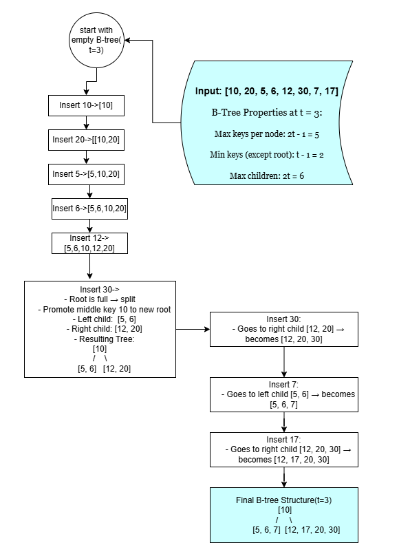
1] B-Trees
What it is?
A self-balancing tree data structure that maintains sorted data and allows searches, sequential access, insertions, and deletions in logarithmic time.
How does it work?
- Uses multi-way branching and store multiple keys per node, reducing the number of disk reads required.
- Internal nodes act as routing indexes while leaves hold actual data pointers.
- Insert: Traverse to the correct leaf, insert key, split if node overflows.
- Search: Navigate from root using key ranges in nodes.
- Delete: Merge/split nodes to maintain balance.
Workflow
5. Code Snippet
class BTreeNode:
    def __init__(self, t, leaf=False):
        self.t = t  # Minimum degree (defines the range for number of keys)
        self.leaf = leaf
        self.keys = []
        self.children = []

    def traverse(self):
        for i in range(len(self.keys)):
            if not self.leaf:
                self.children[i].traverse()
            print(self.keys[i], end=" ")
        if not self.leaf:
            self.children[-1].traverse()

    def search(self, k):
        i = 0
        while i < len(self.keys) and k > self.keys[i]:
            i += 1
        if i < len(self.keys) and self.keys[i] == k:
            return self
        if self.leaf:
            return None
        return self.children[i].search(k)

    def insert_non_full(self, k):
        i = len(self.keys) - 1
        if self.leaf:
            self.keys.append(0)
            while i >= 0 and k < self.keys[i]:
                self.keys[i + 1] = self.keys[i]
                i -= 1
            self.keys[i + 1] = k
        else:
            while i >= 0 and k < self.keys[i]:
                i -= 1
            i += 1
            if len(self.children[i].keys) == 2 * self.t - 1:
                self.split_child(i, self.children[i])
                if k > self.keys[i]:
                    i += 1
            self.children[i].insert_non_full(k)

    def split_child(self, i, y):
        t = self.t
        z = BTreeNode(t, y.leaf)
        z.keys = y.keys[t:]  # Last t-1 keys go to new node
        y.keys = y.keys[:t - 1]  # First t-1 keys remain
        if not y.leaf:
            z.children = y.children[t:]
            y.children = y.children[:t]
        self.children.insert(i + 1, z)
        self.keys.insert(i, y.keys.pop())

class BTree:
    def __init__(self, t):
        self.t = t
        self.root = BTreeNode(t, leaf=True)

    def traverse(self):
        if self.root:
            self.root.traverse()
            print()

    def search(self, k):
        return self.root.search(k)

    def insert(self, k):
        root = self.root
        if len(root.keys) == 2 * self.t - 1:
            temp = BTreeNode(self.t, leaf=False)
            temp.children.insert(0, root)
            temp.split_child(0, root)
            i = 0
            if temp.keys[0] < k:
                i += 1
            temp.children[i].insert_non_full(k)
            self.root = temp
        else:
            root.insert_non_full(k)


if __name__ == '__main__':
    print("B-tree with t=3 (min degree)")
    btree = BTree(t=3)

    values = [10, 20, 5, 6, 12, 30, 7, 17]
    for val in values:
        btree.insert(val)

    print("Traversal of the B-tree:")
    btree.traverse()

    key = 6
    result = btree.search(key)
    print(f"\nSearch for {key}:", "Found" if result else "Not found")


OUTPUT:
B-tree with t=3 (min degree)
Traversal of the B-tree:
5 6 7 12 17 20 30

Search for 6: Found
Efficiency Analysis
- Time: O(log n) for search, insert, delete
- Space: O(1)-Efficient for disk storage due to fewer reads
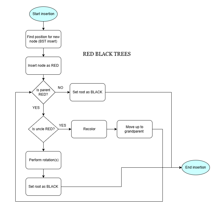
2] Red Black Trees
What it is?
A self-balancing binary search tree where each node has a color (red/black) to enforce balance rules.
How does it work?
- Each node is either red or black.
- Root node is black.
- All Leaf(NIL) nodes are black.
- If a node is red, then both its children are black.
- For each node, every path to a NIL node has the same number of black nodes.
Workflow
5. Code Snippet
RED = True
BLACK = False

class Node:
    def __init__(self, key, color=RED, left=None, right=None, parent=None):
        self.key = key
        self.color = color
        self.left = left
        self.right = right
        self.parent = parent

class RedBlackTree:
    def __init__(self):
        self.NIL = Node(key=None, color=BLACK)  # Sentinel NIL node
        self.root = self.NIL

    def search(self, key, node=None):
        node = node or self.root
        while node != self.NIL and key != node.key:
            node = node.left if key < node.key else node.right
        return node if node != self.NIL else None

    def left_rotate(self, x):
        y = x.right
        x.right = y.left
        if y.left != self.NIL:
            y.left.parent = x
        y.parent = x.parent
        if not x.parent:
            self.root = y
        elif x == x.parent.left:
            x.parent.left = y
        else:
            x.parent.right = y
        y.left = x
        x.parent = y

    def right_rotate(self, x):
        y = x.left
        x.left = y.right
        if y.right != self.NIL:
            y.right.parent = x
        y.parent = x.parent
        if not x.parent:
            self.root = y
        elif x == x.parent.right:
            x.parent.right = y
        else:
            x.parent.left = y
        y.right = x
        x.parent = y

    def insert(self, key):
        node = Node(key)
        node.left = node.right = self.NIL
        parent = None
        current = self.root

        while current != self.NIL:
            parent = current
            current = current.left if node.key < current.key else current.right

        node.parent = parent
        if not parent:
            self.root = node
        elif node.key < parent.key:
            parent.left = node
        else:
            parent.right = node

        node.color = RED
        self.fix_insert(node)

    def fix_insert(self, node):
        while node != self.root and node.parent.color == RED:
            if node.parent == node.parent.parent.left:
                uncle = node.parent.parent.right
                if uncle.color == RED:
                    node.parent.color = BLACK
                    uncle.color = BLACK
                    node.parent.parent.color = RED
                    node = node.parent.parent
                else:
                    if node == node.parent.right:
                        node = node.parent
                        self.left_rotate(node)
                    node.parent.color = BLACK
                    node.parent.parent.color = RED
                    self.right_rotate(node.parent.parent)
            else:
                uncle = node.parent.parent.left
                if uncle.color == RED:
                    node.parent.color = BLACK
                    uncle.color = BLACK
                    node.parent.parent.color = RED
                    node = node.parent.parent
                else:
                    if node == node.parent.left:
                        node = node.parent
                        self.right_rotate(node)
                    node.parent.color = BLACK
                    node.parent.parent.color = RED
                    self.left_rotate(node.parent.parent)
        self.root.color = BLACK

    def inorder(self, node=None):
        node = node or self.root
        if node == self.NIL:
            return
        self.inorder(node.left)
        print(node.key, end=' ')
        self.inorder(node.right)

# Example usage
if __name__ == "__main__":
    tree = RedBlackTree()
    values = [10, 20, 30, 15, 25, 5, 1]
    for val in values:
        tree.insert(val)

    print("In-order traversal of Red-Black Tree:")
    tree.inorder()

    key = 15
    found = tree.search(key)
    print(f"\nSearch for {key}:", "Found" if found else "Not Found")

OUTPUT:
In-order traversal of Red-Black Tree:
1 5 10 15 20 25 30
Search for 15: Found
Efficiency Analysis
- Time:O(log n) for all operations
- Space:O(n)-Efficient, requires storing color bits
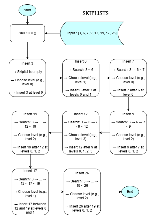
3] Skiplists
What it is?
A probabilistic data structure that maintains elements in sorted order using multiple levels of linked lists.
How does it work?
- Skiplist is a multi-level linked list for fast search.
- Each node’s level is chosen randomly (usually with a probability p = 0.5), determining how many levels it spans.
- Insertion places the node in all its levels.
- Search starts from the top level and drops down.
- Deletion removes the node from all its levels.
Workflow
5. Code Snippet
import random

MAX_LEVEL = 4  # max levels in skiplist

class Node:
    def __init__(self, key, level):
        self.key = key
        self.forward = [None] * (level + 1)

class Skiplist:
    def __init__(self):
        self.header = Node(-1, MAX_LEVEL)
        self.level = 0

    def random_level(self):
        lvl = 0
        while random.random() < 0.5 and lvl < MAX_LEVEL:
            lvl += 1
        return lvl

    def insert(self, key):
        update = [None] * (MAX_LEVEL + 1)
        current = self.header

        # Start from highest level and move forward
        for i in range(self.level, -1, -1):
            while current.forward[i] and current.forward[i].key < key:
                current = current.forward[i]
            update[i] = current

        current = current.forward[0]

        # Insert if not present
        if current is None or current.key != key:
            lvl = self.random_level()

            if lvl > self.level:
                for i in range(self.level + 1, lvl + 1):
                    update[i] = self.header
                self.level = lvl

            new_node = Node(key, lvl)
            for i in range(lvl + 1):
                new_node.forward[i] = update[i].forward[i]
                update[i].forward[i] = new_node

    def search(self, key):
        current = self.header
        for i in range(self.level, -1, -1):
            while current.forward[i] and current.forward[i].key < key:
                current = current.forward[i]

        current = current.forward[0]
        if current and current.key == key:
            return True
        return False

    def display(self):
        for i in range(self.level + 1):
            current = self.header.forward[i]
            print(f"Level {i}: ", end="")
            while current:
                print(current.key, end=" -> ")
                current = current.forward[i]
            print("None")

# Usage
skiplist = Skiplist()
values = [3, 6, 7, 9, 12, 19, 17, 26]
for val in values:
    skiplist.insert(val)

print("Skiplist structure:")
skiplist.display()

print("\nSearch 19:", "Found" if skiplist.search(19) else "Not Found")
print("Search 15:", "Found" if skiplist.search(15) else "Not Found")


OUTPUT:
Skiplist structure:
Level 0: 3 -> 6 -> 7 -> 9 -> 12 -> 17 -> 19 -> 26 -> None
Level 1: 3 -> 12 -> 26 -> None
Level 2: 3 -> 26 -> None
Level 3: 3 -> None

Search 19: Found
Search 15: Not Found
Efficiency Analysis
- Time: O(log n) average, O(n) worst
- Space:O(nlog n) average, O(n) worst
Case Study Summary
| Sl.no. | Algorithm | Time Complexity (Prefix Query) | Space Efficiency | Notable Difference | Suitability for Use Case: data storage and indexing |
|---|---|---|---|---|---|
| 1 | B-Trees | O(log n) | High (disk/page optimized) | Balanced multi-way tree ideal for large disk-based data structures. | Widely used in databases and filesystems (e.g., Google’s Bigtable). |
| 2 | Red-Black Trees | O(log n) | Moderate | Self-balancing binary tree with strict color and rotation rules. | Efficient for in-memory indexing with consistent performance. |
| 3 | Skiplists | O(log n) | Moderate (more pointers per node) | Randomized level-based linked structure enabling fast traversal. | Good for concurrent systems like Google’s LevelDB. |
Case 4: Real-Time Analytics and Monitoring
1. Business Problem Statement
To track, update, and analyze massive volumes of user interactions (clicks, views, impressions) in real-time to deliver actionable insights and personalized experiences.
Domain: Real-Time Data Processing, Streaming Analytics, AdTech, Recommendation Systems
2. Challenges
- Processing millions of user events per second with minimal latency.
- Efficiently updating and querying time-series metrics (clicks, views) in real-time.
- Handling dynamic data where frequent updates and fast range queries are essential.
- Balancing performance and memory usage for high-frequency analytics.
3. Algorithms Involved
- Fenwick Trees (Binary Indexed Trees) – allow efficient prefix sum and point update operations in logarithmic time, ideal for time-series tracking (e.g., total clicks till time T).
- Segment Trees – support complex range queries (sum, max, min, etc.) and range updates with lazy propagation for advanced analytics and summarization.
- Hashing Algorithms – used to map user IDs, session tokens, or page categories for quick aggregation and lookup.
- Sliding Window & Streaming Algorithms – used in conjunction to maintain statistics over recent time intervals (e.g., last 10 minutes of views).
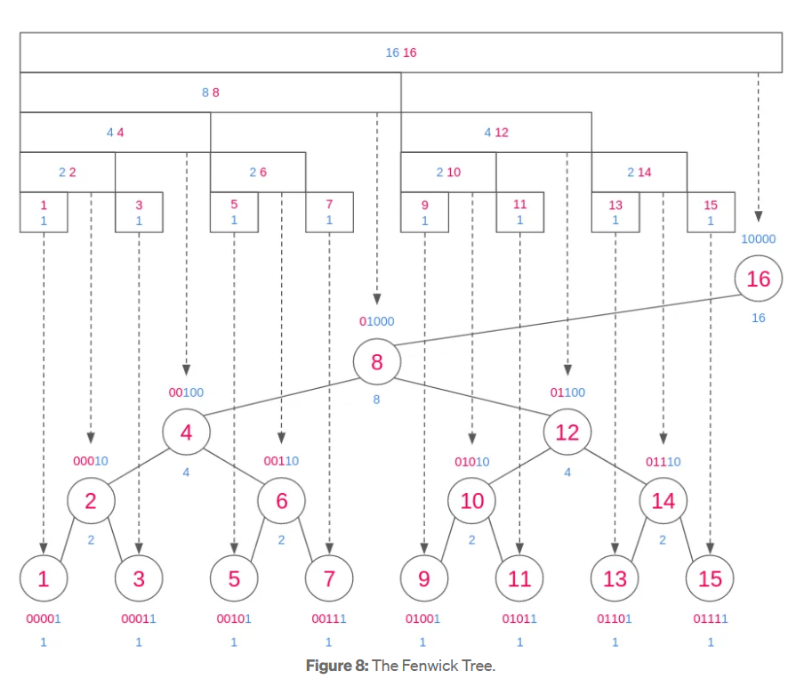
1] Fenwick Trees (Binary Indexed Trees)
What it is?
A data structure that provides efficient methods for calculation and manipulation of prefix sums in a list of numbers. It's widely used in frequency tables, time-series analysis, and competitive programming.
How does it work?
- Stores cumulative frequency data in a tree-like structure using bit manipulation.
- Each index holds the sum of a specific range of elements from the input array.
- Update: Modify element and update relevant tree indices using `index += index & -index`.
- Query: Get prefix sum up to a certain index using `index -= index & -index`.
- Efficient for dynamic data with frequent updates and queries.
Workflow
5. Code Snippet
class FenwickTree:
    def __init__(self, size):
        # Size of the array (1-based indexing)
        self.n = size
        self.tree = [0] * (size + 1)

    def update(self, index, delta):
        """Add `delta` to element at `index` (1-based)."""
        while index <= self.n:
            self.tree[index] += delta
            index += index & -index  # Move to next responsible node

    def query(self, index):
        """Get prefix sum from index 1 to `index`."""
        result = 0
        while index > 0:
            result += self.tree[index]
            index -= index & -index  # Move to parent
        return result

    def range_query(self, left, right):
        """Get sum of range [left, right]."""
        return self.query(right) - self.query(left - 1)


# Example usage
if __name__ == '__main__':
    print("Fenwick Tree Example")
    values = [3, 2, -1, 6, 5, 4, -3, 3, 7, 2]  # 10 elements

    ft = FenwickTree(len(values))
    for i, val in enumerate(values):
        ft.update(i + 1, val)  # Update using 1-based index
    print("Array:",values)
    print("Prefix sum up to index 5 (1 based indexing):", ft.query(5))       # Should output 15
    print("Range sum from index 3 to 7 (1 based indexing):", ft.range_query(3, 7))  # Should output 11

OUTPUT:
Fenwick Tree Example
Array: [3, 2, -1, 6, 5, 4, -3, 3, 7, 2]
Prefix sum up to index 5 (1 based indexing): 15
Range sum from index 3 to 7 (1 based indexing): 11
Efficiency Analysis
- Time: O(log n) for update and prefix sum queries
- Space: O(n) additional storage for tree array
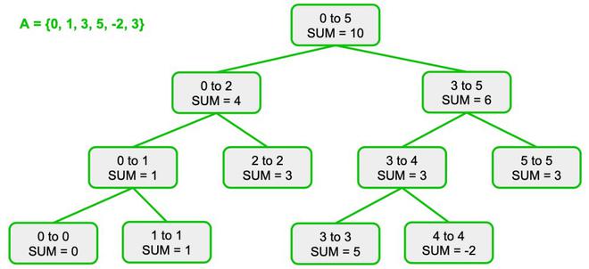
2] Segment Trees
What it is?
A segment tree is a binary tree used for storing intervals or segments. It allows answering range queries and updates over an array efficiently. Common operations include sum, min, max, GCD over a range, etc.
How does it work?
- Build: Recursively divide the array into halves and build the tree bottom-up.
- Each internal node stores an aggregate value (e.g., sum or min) of its children.
- Query: Use divide-and-conquer to check how much of the current segment overlaps with the query range.
- Update: Traverse down to the affected leaf node and propagate changes upwards.
- More powerful than Fenwick trees: supports range updates and more complex operations.
Workflow
5. Code Snippet
class SegmentTree:
    def __init__(self, data):
        self.n = len(data)
        self.tree = [0] * (4 * self.n)
        self.build(data, 0, 0, self.n - 1)

    def build(self, data, node, start, end):
        if start == end:
            self.tree[node] = data[start]
        else:
            mid = (start + end) // 2
            self.build(data, 2 * node + 1, start, mid)
            self.build(data, 2 * node + 2, mid + 1, end)
            self.tree[node] = self.tree[2 * node + 1] + self.tree[2 * node + 2]

    def update(self, idx, value, node=0, start=0, end=None):
        if end is None: end = self.n - 1
        if start == end:
            self.tree[node] = value
        else:
            mid = (start + end) // 2
            if idx <= mid:
                self.update(idx, value, 2 * node + 1, start, mid)
            else:
                self.update(idx, value, 2 * node + 2, mid + 1, end)
            self.tree[node] = self.tree[2 * node + 1] + self.tree[2 * node + 2]

    def query(self, l, r, node=0, start=0, end=None):
        if end is None: end = self.n - 1
        if r < start or l > end:
            return 0
        if l <= start and end <= r:
            return self.tree[node]
        mid = (start + end) // 2
        left = self.query(l, r, 2 * node + 1, start, mid)
        right = self.query(l, r, 2 * node + 2, mid + 1, end)
        return left + right

# Example usage
if __name__ == '__main__':
    print("Segment Tree Example")
    data = [3, 2, -1, 6, 5, 4, -3, 3, 7, 2]
    st = SegmentTree(data)
    print("Array:", data)
    print("Sum from index 0 to 4:", st.query(0, 4))   # Output: 15
    print("Sum from index 3 to 7:", st.query(3, 7))   # Output: 15
    st.update(3, 10)  # Update index 3 to 10
    print("After update at index 3 to 10:")
    print("Sum from index 3 to 7:", st.query(3, 7))   # Output should reflect updated value

OUTPUT:
Segment Tree Example
Array: [3, 2, -1, 6, 5, 4, -3, 3, 7, 2]
Sum from index 0 to 4: 15
Sum from index 3 to 7: 15
After update at index 3 to 10:
Sum from index 3 to 7: 19
Efficiency Analysis
- Time: O(log n) for query and update operations
- Space: O(4n) for tree storage (safe upper bound)
Case Study Summary
| Sl.no. | Algorithm | Time Complexity (Prefix Query) | Space Efficiency | Notable Difference | Suitability for Use Case: Real-Time Monitoring and Analytics |
|---|---|---|---|---|---|
| 1 | Fenwick Trees (Binary Indexed Trees) | O(log n) | High (O(n)) | Efficient for dynamic prefix sums and updates using bit manipulation. | Ideal for fast incremental updates and prefix queries in streaming data (e.g., tracking real-time event counts). |
| 2 | Segment Trees | O(log n) | Moderate to High (O(2n)) | Supports a wider range of range queries (sum, min, max) and updates. | Used when complex interval queries and dynamic updates are needed in large-scale analytics. |
Case 5: Content Ranking and Personalization
1. Business Problem Statement
To rank billions of web pages and content items effectively and personalize recommendations by identifying relevant, popular, and similar content in real-time.
Domain: Search Engines, Recommendation Systems, Personalization, AdTech
2. Challenges
- Handling massive web graphs with billions of pages and links.
- Ranking pages based on authority and relevance efficiently.
- Tracking frequently popular content with space constraints.
- Personalizing recommendations by identifying similar items in large high-dimensional data.
- Balancing accuracy, latency, and scalability for real-time personalization.
3. Algorithms Involved
- PageRank – Calculates a global ranking score for each page based on the link structure of the web, representing page importance.
- Space-Saving Algorithm – Efficiently tracks top-k frequent items in a data stream with bounded memory, useful for popular content tracking.
- Locality-Sensitive Hashing (LSH) – Quickly identifies similar items by hashing high-dimensional data to buckets, enabling fast personalized recommendations.
1] PageRank Algorithm
What it is?
A link analysis algorithm that assigns a numerical weight to each element of a hyperlinked set of documents to measure its relative importance within the set.
How does it work?
- Represents the web as a directed graph where pages are nodes and hyperlinks are edges.
- Pages pass "rank" scores to linked pages proportionally.
- Uses an iterative approach with damping factor to model random surfing behavior.
- Converges when ranks stabilize, indicating page importance.
Workflow
5. Code Snippet (Simplified Python)
def pagerank(graph, damping=0.85, max_iter=100, tol=1e-6):
    nodes = list(graph.keys())
    n = len(nodes)
    rank = {node: 1 / n for node in nodes}

    for _ in range(max_iter):
        prev_rank = rank.copy()
        for node in nodes:
            incoming = [src for src in nodes if node in graph[src]]
            rank[node] = (1 - damping) / n + damping * sum(
                prev_rank[src] / len(graph[src]) for src in incoming
            )
        # Check convergence
        if all(abs(rank[node] - prev_rank[node]) < tol for node in nodes):
            break

    return rank

# Example graph
graph = {
    'A': ['B', 'C'],
    'B': ['C'],
    'C': ['A'],
    'D': ['C']
}

ranks = pagerank(graph)

# Sort and print ranks in descending order
sorted_ranks = sorted(ranks.items(), key=lambda x: x[1], reverse=True)

print("Final Ranking Order:")
for i, (node, score) in enumerate(sorted_ranks, 1):
    print(f"{i}. {node} ({score:.4f})")

# Optional: get just the order string
rank_order = " > ".join(node for node, _ in sorted_ranks)
print("Rank Order:", rank_order)


OUTPUT:
Final Ranking Order:
1. C (0.3941)
2. A (0.3725)
3. B (0.1958)
4. D (0.0375)
Rank Order: C > A > B > D
Efficiency Analysis
- Time: O(k * (V + E)) where k is iterations, V vertices, E edges
- Space: O(V + E) to store graph and ranks
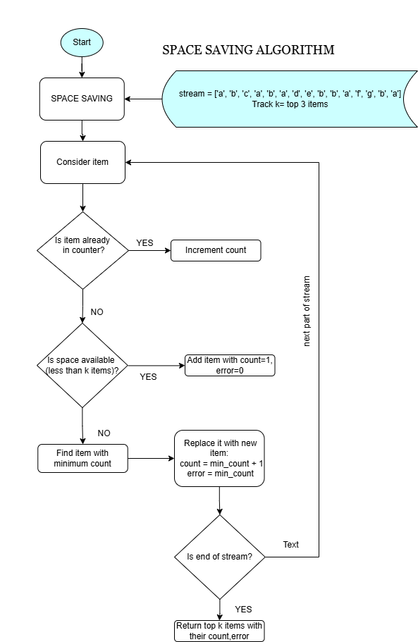
2] Space-Saving Algorithm
What it is?
An algorithm to track the top-k most frequent elements in a stream efficiently with fixed memory, allowing approximate frequency counts with error bounds.
How does it work?
- Maintains a fixed-size summary data structure for the top-k items.
- For each new item, if it exists in the summary, increment count; else, replace the minimum count item.
- Ensures frequent items are retained, and infrequent ones are discarded.
Workflow
5. Code Snippet (Simplified Python)
from collections import defaultdict

class SpaceSaving:
    def __init__(self, k):
        self.k = k  # Maximum number of elements to track
        self.counters = {}  # Dictionary to store item -> (count, error)

    def process(self, item):
        if item in self.counters:
            self.counters[item][0] += 1  # Increment count
        elif len(self.counters) < self.k:
            self.counters[item] = [1, 0]  # New item, no error
        else:
            # Find item with minimum count
            min_item = min(self.counters.items(), key=lambda x: x[1][0])
            min_key, (min_count, _) = min_item
            # Replace with new item, inherit min_count as error
            del self.counters[min_key]
            self.counters[item] = [min_count + 1, min_count]

    def get_frequent_items(self):
        return sorted(
            ((item, count, error) for item, (count, error) in self.counters.items()),
            key=lambda x: -x[1]
        )

# Example usage
if __name__ == '__main__':
    stream = ['a', 'b', 'c', 'a', 'b', 'a', 'd', 'e', 'b', 'b', 'a', 'f', 'g', 'b', 'a']
    ss = SpaceSaving(k=3)  # Track top-3 frequent items

    for item in stream:
        ss.process(item)

    print("Top-k Frequent Items (Item, Estimated Count, Error):")
    for entry in ss.get_frequent_items():
        print(entry)

OUTPUT:
Top-k Frequent Items (Item, Estimated Count, Error):
('b', 5, 2)
('g', 5, 4)
('a', 5, 4)
Efficiency Analysis
- Time: O(log k) per update (if using heap or balanced tree)
- Space: O(k) fixed memory footprint
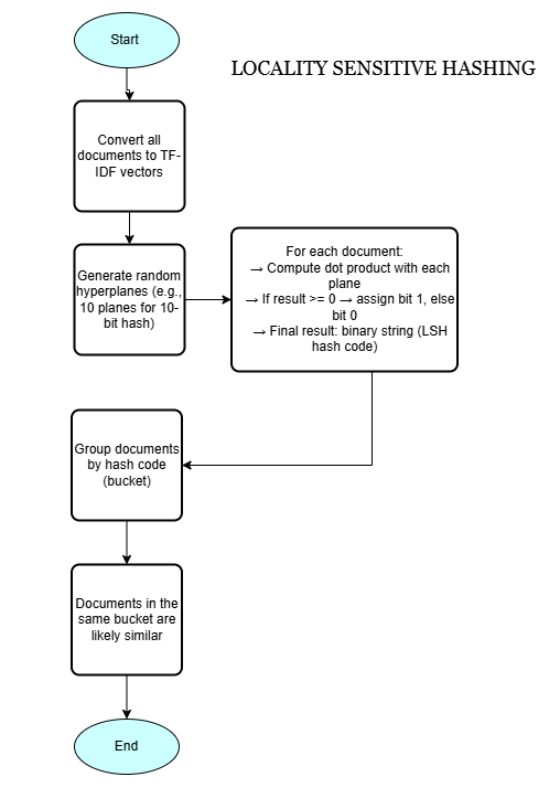
3] Locality-Sensitive Hashing (LSH)
What it is?
A probabilistic hashing technique designed to hash similar input items into the same buckets with high probability, enabling fast approximate nearest neighbor search in high-dimensional spaces.
How does it work?
- Transforms high-dimensional vectors (e.g., user profiles, document features) into buckets.
- Uses hash functions sensitive to input similarity (e.g., cosine similarity, Jaccard similarity).
- Similar items collide in buckets, allowing efficient approximate similarity search.
- Enables fast personalized recommendations by identifying similar content/users.
Workflow
5. Code Snippet (Simplified Python using MinHash for Jaccard)
import numpy as np
from sklearn.feature_extraction.text import TfidfVectorizer

class LSH:
    def __init__(self, num_hashes, dim):
        self.num_hashes = num_hashes
        self.planes = np.random.randn(num_hashes, dim)  # Random hyperplanes

    def hash(self, vector):
        # Compute dot product with each plane and get 1 if >=0 else 0
        return ''.join(['1' if np.dot(vector, plane) >= 0 else '0' for plane in self.planes])

# Sample documents
docs = [
    "the cat sat on the mat",
    "the cat sat on a mat",
    "dogs are in the yard",
    "the quick brown fox jumps over the lazy dog"
]

# Step 1: TF-IDF vectorization
vectorizer = TfidfVectorizer()
tfidf_matrix = vectorizer.fit_transform(docs).toarray()

# Step 2: Hash documents using LSH
lsh = LSH(num_hashes=10, dim=tfidf_matrix.shape[1])
buckets = {}

for idx, vec in enumerate(tfidf_matrix):
    h = lsh.hash(vec)
    if h not in buckets:
        buckets[h] = []
    buckets[h].append((idx, docs[idx]))

# Step 3: Show buckets with near-duplicates
print("Buckets with near-duplicate documents:")
for bucket, items in buckets.items():
    if len(items) > 1:
        print(f"\nBucket Hash: {bucket}")
        for i in items:
            print(f"Doc {i[0]}: {i[1]}")


OUTPUT:
Buckets with near-duplicate documents:

Bucket Hash: 0010010101
Doc 0: the cat sat on the mat
Doc 1: the cat sat on a mat
Code result analysis
- Bucket Hash
1010100110is created by projecting document vectors onto random hyperplanes and encoding signs as bits. - Documents 0 and 1 share the same bucket hash, indicating very similar vector representations (near-duplicates).
- Other documents have different hashes, meaning they are dissimilar and placed in separate buckets.
- LSH groups similar items into the same bucket with high probability, enabling fast similarity detection.
- This avoids costly all-pairs comparisons by limiting comparisons to items within the same bucket.
- Documents about “cat sat on the mat” are recognized as similar and grouped together in the output.
Efficiency Analysis
- Time: O(num_hashes) for signature, O(1) average bucket lookup
- Space: O(num_bands * bucket size), efficient for large-scale high-dimensional data
Case Study Summary
| Sl.no. | Algorithm | Time Complexity | Space Efficiency | Notable Difference | Suitability for Use Case: Content Ranking and Personalization |
|---|---|---|---|---|---|
| 1 | PageRank | O(k * (V + E)) | High (O(V + E)) | Iterative link analysis algorithm for global page importance. | Effective for ranking billions of web pages by authority and relevance. |
| 2 | Space-Saving Algorithm | O(log k) | Fixed (O(k)) | Approximate top-k frequency tracking in streams with error bounds. | Used for monitoring popular content and keywords efficiently in large data streams. |
| 3 | Locality-Sensitive Hashing (LSH) | O(num_hashes) | Moderate | Probabilistic hashing to group similar items in buckets for fast similarity search. | Enables real-time personalized recommendations based on content/user similarity. |